The Gibbs phenomenon

I remember that my undergrad teacher once said that “The Gibbs phenomenon is there to remind you of the uniform limit theorem”. That is, a Fourier series can’t converge uniformly to a discontinuous function. The Wikipedia page has a great overview of the phenomenon with both math and signal processing explanations.

Let us look at the simple example of

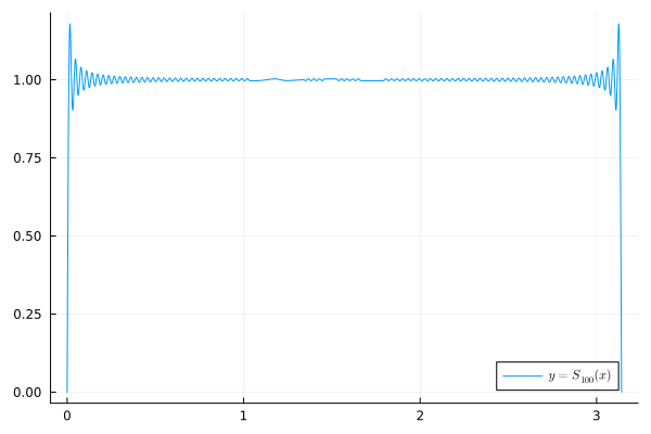
Which converge (in the $L^2$ norm) to $1$ on $[0,\pi]$. However, if we take any partial sum, we see some wiggles at the endpoints. For example, here’s the sum of the first 100 terms

S(m,x) = 4/pi*sum(sin((2k-1)*x)/(2k-1) for k=1:m)


plot(x->S(100,x),0,pi,label=L"y=S_{100}(x)")

One possible way to fix it is by using a Cesàro summation (In the case of Fourier series it leads to Fejer’s kernel):

This will reduce the oscillations, here’s a plot of $T_{100}$ 

Fejer(m,x) = 4/pi*sum((1-(2k-1)/(2m-1))sin((2k-1)*x)/(2k-1) for k=1:m)

plot(x->Fejer(100,x),0,pi)

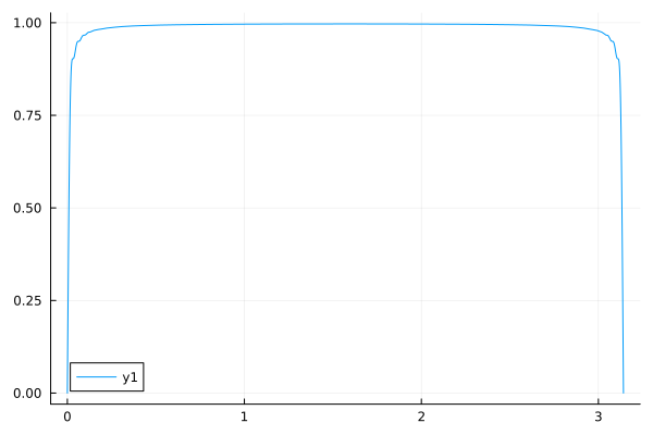
The drawback of Fejer’s Kernel is that we lose some accuracy at the boundaries. A “sometimes” better alternative, is the Lanczos sigma factor, where instead of $1-\frac{2k-1}{2m-1}$, we use $[\text{sinc}\left(\frac{2k-1}{2m-1}\right)]^{\alpha}$ where $\text{sinc}(x)=\frac{\sin(\pi x)}{\pi x}$ and $\alpha\ge 1$. Here’s an example with $\alpha=3$ 

Lanc(m,x,α) = 4/pi*sum(sinc((2k-1)/(2m-1))^α * sin((2k-1)*x)/(2k-1) for k=1:m)
plot(x->Lanc(100,x,3),0,pi)

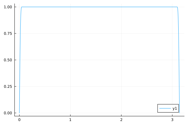
This is clearly better than what we obtained using Fejer’s kernel. To see why the Sigma factor outperformed Fejer’s kernel, we need to look at the plots of $1-z$ and $\text{sinc}(z)^{\alpha}$ for $0\le z\le 1$: 

plot(z->1-z,0,1,label=L"1-z")
plot!(z->sinc(z),0,1,label=L"\operatorname{sinc}(z)")
plot!(z->sinc(z)^2,0,1,label=L"\operatorname{sinc}(z)^2")
plot!(z->sinc(z)^3,0,1,label=L"\operatorname{sinc}(z)^3")

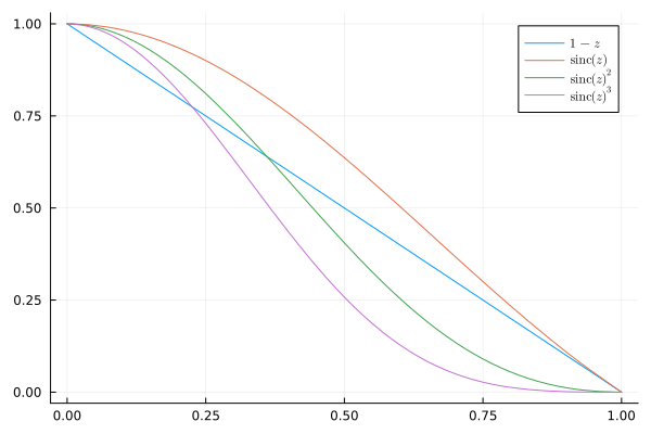
The values of $z$ that are close to zero correspond to low value of $k$ (think of $z$ as $\frac{2k-1}{2m-1}$). We can see that what the sigma factor is doing differently is that it keeps the low frequency coefficients (low k) roughly the same and makes the high frequency coefficients smaller (especially when $\alpha=2,3$).

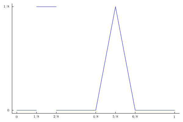
Here’s what led me through this rabbit hole? I gave my students the following wave equation as homework.

where $f$ looks like this: 

plot([0/8,1/8],[0,0],c=:blue,legend=false,yticks=([0,1/8],[L"0",L"1/8"]),
    xticks=([0,1,2,4,5,6,8]/8, [L"0",L"1/8",L"2/8",L"4/8",L"5/8",L"6/8",L"1"]),
    grid=false
    )
plot!([1,2]/8,[1,1]/8,c=:blue)
plot!([2,4]/8,[0,0]/8,c=:blue)
plot!([4,5]/8,[0,1]/8,c=:blue)
plot!([5,6]/8,[1,0]/8,c=:blue)
plot!([6,8]/8,[0,0]/8,c=:blue)

If we just plot the first few terms of the Fourier series representation of the solution, we will see the Gibbs phenomenon for all times $t$ no matter how many terms we use: 

A(n)=-sin(n*π/16)^2*(π*n+16*sin(5π*n/8)+2π*n*cos(n*π/8))/(2*π^2*n^2)
u1(x,t)=sum(A(n)*sin(n*π*x)*(cos(n*π*t)-1/(n*π)*sin(n*π*t)) for n=1:100)

anim1 = @animate for t in range(0,2,200)
               plot(x->u1(x,t),0,1,c=:blue,legend=false,yticks=([-1/8,0,1/8],[L"-1/8",L"0",L"1/8"]),
                xticks=([0,1], [L"0",L"1"]),ylims=(-1.1/8,1.1/8),
                grid=false)
        end

gif(anim1, "anim1.gif", fps = 15)

If we use a sigma-factor of $3$, we see that the Gibbs phenomenon disappears (at least visually): 

A(n)=-sin(n*π/16)^2*(π*n+16*sin(5π*n/8)+2π*n*cos(n*π/8))/(2*π^2*n^2)
u2(x,t)=sum(sinc(n/100)^3*A(n)*sin(n*π*x)*(cos(n*π*t)-1/(n*π)*sin(n*π*t)) for n=1:100)

anim2 = @animate for t in range(0,2,200)
               plot(x->u2(x,t),0,1,c=:blue,legend=false,yticks=([-1/8,0,1/8],[L"-1/8",L"0",L"1/8"]),
                xticks=([0,1], [L"0",L"1"]),ylims=(-1.1/8,1.1/8),
                grid=false)
        end